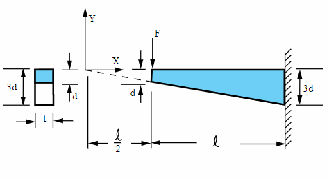
Laterally loaded tapered support structure (Shell element)¤

This live script is written as a guided walkthrough for a verification benchmark. It compares a known structural response with the result produced by the OpenSeesMatlab workflow. Read the text cells first, then run each code cell in order so that the variables, model state, and recorded results are available for the later sections.

See Laterally loaded tapered support structure — PyMAPDL Examples

Shell element in OpenSees

clear; clc;

Output

[OpenSeesMatlab]  [EXCEPTION] Polyscope has not been initialized

%% Get OpenSeesMatlab instance
opsMAT = OpenSeesMatlab();
ops = opsMAT.opensees;

FE Model¤

This section creates the finite-element idealization used by the rest of the example. Check the dimensions, tags, and connectivity here before moving on.

%% Clean model
ops.wipe();
ops.model('basic', '-ndm', 3, '-ndf', 6);

%% Material and thickness
E  = 30e6;    % psi
nu = 0.0;
t  = 2.0;     % in

matTag = 1;
ops.nDMaterial('ElasticIsotropic', matTag, E, nu);
secTag = 1;
ops.section('PlateFiber', secTag, matTag, t);

%% Mesh control
nElem = 50;          % number of quad elements along the beam length
nNodePerEdge = nElem + 1;

%% Geometry
% Top edge:    from (25,  0) to (75,  0)
% Bottom edge: from (25, -3) to (75, -9)

xTop = linspace(25, 75, nNodePerEdge);
yTop = zeros(1, nNodePerEdge);

xBot = linspace(25, 75, nNodePerEdge);
yBot = linspace(-3, -9, nNodePerEdge);

% Node numbering:
% top    : 1 ~ nNodePerEdge
% bottom : nNodePerEdge+1 ~ 2*nNodePerEdge

for i = 1:nNodePerEdge
    ops.node(i, xTop(i), 0.0, yTop(i));
end

for i = 1:nNodePerEdge
    ops.node(nNodePerEdge + i, xBot(i), 0.0, yBot(i));
end

%% Elements
% Counterclockwise ordering:
% [bottom-left, bottom-right, top-right, top-left]

conn = zeros(nElem, 4);

for e = 1:nElem
    nBL = nNodePerEdge + e;
    nBR = nNodePerEdge + e + 1;
    nTR = e + 1;
    nTL = e;

    conn(e, :) = [nBL, nBR, nTR, nTL];

    % ops.element('quad', e, nBL, nBR, nTR, nTL, t, 'PlaneStress', matTag);
    % ops.element('ShellMITC4', e, nBL, nBR, nTR, nTL, secTag);
    ops.element('ASDShellQ4', e, nBL, nBR, nTR, nTL, secTag);  % Better than ShellMITC4
end

Output

[OpenSees] Using ASDShellQ4 - Developed by: Massimo Petracca, Guido Camata, ASDEA Software Technology

%% Boundary conditions
% Fixed end at x = 75 -> top last node and bottom last node
topFixed = nNodePerEdge;
botFixed = 2 * nNodePerEdge;

ops.fix(topFixed, 1, 1, 1, 1, 1, 1);
ops.fix(botFixed, 1, 1, 1, 1, 1, 1);

%% Load
% Concentrated vertical load at top-left node
ops.timeSeries('Linear', 1);
ops.pattern('Plain', 1, 1);
ops.load(1, 0.0, 0.0, -4000.0, 0.0, 0.0, 0.0);

Plot Model¤

This section creates the finite-element idealization used by the rest of the example. Check the dimensions, tags, and connectivity here before moving on.

opts = opsMAT.vis.defaultPlotModelOptions;
opts.nodes.showLabels = false;
opts.elements.showLabels = false;
opts.loads.showNodal = true;
opsMAT.vis.plotModel(opts=opts);

Output

[OpenSeesMatlab] Model summary
  Nodes: 102
  Shell elements: 50

view([0 0]);
grid off

Analysis setup¤

This section configures and runs the analysis. The solver, constraints, convergence test, and step size should be read together because they control numerical robustness.

Nsteps = 2;
ops.constraints('Plain');
ops.numberer('RCM');
ops.system('BandGeneral');
ops.test('NormDispIncr', 1.0e-12, 50);
ops.algorithm('Newton');
ops.integrator('LoadControl', 1.0 / Nsteps);
ops.analysis('Static');

ODB = opsMAT.post.createODB("myODB", projectGaussToNodes="extrapolate");  % create ODB

Output

Output file: .openseesmatlab.output\Responses-myODB.odb\output.h5

ok = ops.analyze(Nsteps);
ODB.close();

Post-processing¤

The following commands carry out this step of the workflow. Run this cell after the previous sections so the required variables and model state already exist.

nodeResp = opsMAT.post.getNodalResponse("myODB");

opts = opsMAT.vis.defaultPlotNodalResponseOptions;
opts.fixed.show = true;
opts.surf.showEdges = false;
opts.deform.show = true;

opsMAT.vis.plotNodalResponse(nodeResp, respType="disp", stepIdx="absMax", respComponent="UZ", opts=opts);
colormap("jet")
axis off
view([0 0]);
grid off
title("Displacement Along y-Direction")

shellResp = opsMAT.post.getElementResponse("myODB", eleType="Shell");
opsMAT.vis.plotShellResponse(shellResp, ...
    respType="StressAtNode", fiberPoint='top', respComponent="sxx", opts=opts);
axis off
grid off
view([0 0]);
title("Sxx Stress");

opsMAT.vis.plotShellResponseGUI(shellResp);

sxx = shellResp.StressAtNode.sxx;   % sxx

nodeTags = shellResp.nodeTags;

Find nodes closest to (75,0) and (50,0)

numNode = 2 * nNodePerEdge;
coords = zeros(numNode, 2);
for i = 1:nNodePerEdge
    coords(i, :) = [xTop(i), yTop(i)];
end
for i = 1:nNodePerEdge
    coords(nNodePerEdge + i, :) = [xBot(i), yBot(i)];
end

fixedNode = localFindNearestNode(coords, [75, 0]);

fixedIdx = nodeTags == fixedNode;

% get stress
sxxFixed = sxx(:, fixedIdx, :);  % nStep * nFiber
fixed_end_stress_osp = max(sxxFixed(:));

%% Reference values from ANSYS example
target_end = 7407.0;
mapdl182_end = 7151.10;

Comparing the results, note that ANSYS only used 7 elements, so the results will be somewhat worse. However, if OpenSees also uses 7 elements, the results are surprisingly poor!

fprintf('end sigma_x: target = %.2f, MAPDL182 = %.2f, OpenSeesMatlab = %.2f, ratio = %.4f\n', ...
    target_end, mapdl182_end, fixed_end_stress_osp, fixed_end_stress_osp / target_end);

Output

end sigma_x: target = 7407.00, MAPDL182 = 7151.10, OpenSeesMatlab = 7481.59, ratio = 1.0101

Visualization by Polyscope GUI¤

opsMAT.vis.polyscope.plotNodalResponse(nodeResp);

Output

[OpenSeesMatlab] Backend: openGL3_glfw -- Loaded openGL version: 3.3.0 NVIDIA 561.09

opsMAT.vis.polyscope.plotShellResponse(shellResp);

Local function:¤

function nodeId = localFindNearestNode(coords, pt)
    d2 = (coords(:,1) - pt(1)).^2 + (coords(:,2) - pt(2)).^2;
    [~, nodeId] = min(d2);
end